Diamond Version 5 User Manual: Exploring bonding and contact spheres

Exploring bonding spheres

- About bonding spheres, connectivity, and atomic environments
- Starting from a single atom of the parameter list
- Using "Get Molecule" or "Fill Unit Cell"
- Example COD:7106313
- Example antimony trifluoride/pentafluoride adduct (Sb4F16)

Previous article: Working in Exploration View
Next article: Exploring H-bonds and contact spheres

About bonding spheres, connectivity, and atomic environments

Bonding spheres on atom type level

When a structure is read into Diamond or structure parameters are manually entered, the atoms of the atomic parameter list are grouped together in a list of so-called atom groups. By default, atom groups differ by ordinal number and oxidation number, that means the term atom group can be used equivalently with atom type. (We use the special term atom group in Diamond, because atoms belonging to different atom types can manually be grouped together in one atom group. On the other side, different atoms of the parameter list having the same ordinal and oxidation number, if any, can be grouped into different atom groups. See "About atoms, atom groups, bonds, and bond groups".)

For every pair of atom groups (atom types) in a compound, a bond group with a bonding sphere is defined and a flag whether this bonding sphere is active or not, i.e. whether bonds are allowed for this atom type pair or not.

Whenever a structure has been imported or the atomic parameter list has been edited, bond groups will be initialized or reset, rsp. The bonding sphere of a bond group is calculated like this:

If a mean bond value is defined for the element combination of the bond group (ignoring oxidation numbers) in the factory default settings of Diamond or in the Diamond section of the Windows Registry (if you have made changes to the default value), this value is taken as mean value of the bonding sphere. Otherwise, the effective radii of the two atom groups are added.

The result is multiplied with the lower sphere boundary factor to get the lower boundary value of the bonding sphere. The upper sphere boundary factor is used for the upper boundary value. Diamond works with default boundary factors of 0.6 and 1.2, rsp. (To edit the boundary factors, use the Connectivity dialog, opened from the Build -> Connectivity command.)

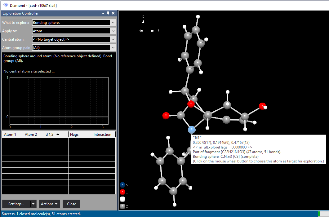
All bond groups are selected, unless the oxidation numbers have the same sign.

Bonding spheres on atom site level
The Atomic environment was introduced in version 4 of Diamond as an additional (optional) criterion when filling a coordination sphere or adding coordination polyhedra. Defining an atomic environment for every atom site makes the search for bonded neighbouring atoms much more flexible than by defining between atom types only. This is especially the case when some of the atom sites belonging to a certain atom type have deviating environments, and a bonding sphere definition in the "Connectivity" dialog does not match all cases. Or the spreading of distances in the histogram of the "Connectivity" dialog makes it difficult to find the (upper) boundary of the bonding sphere for the selected atom type pair there.

The bonding spheres (as part of the "connectivity") and the atomic environments can also be checked and changed using the commands Connectivity and Atomic Environments, rsp., both from the Build menu, in the regular Picture Edit view of Diamond. See the articles "Connectivity, part 1: Bonding spheres" and ""Atomic environment" as additional (optional) criterion when filling a coordination sphere or adding coordination polyhedra".

Starting from a single atom of the parameter list

The simplest case is starting your study of bonding spheres from a single atom of the parameter list as central atom of the sphere (or center of the atomic environment). You may create the (central) atom in the Picture Edit view already and then begin the exploration or enter the exploration with a blank picture and create an atom there using the Add Atom command.

In the first case, this (central) atom will be automatically set as reference atom. When you enter the exploration view with a blank picture, you can choose a reference atom directly from the Central atom dropdown box in the Exploration Controller, where you choose Add atom as target... (since there is no atom yet in the picture to choose from). From the Add Atom dialog choose an atom (you may create multiple atoms, too) to become your center of interest. When confirmed with OK, the atom is added to the structure picture, registered as target object and the atoms and bonds belonging to the current settings of the bonding sphere will be created, too.

Note: You can also start an exploration from a (manually or semi-automatically) built up structure picture. See the article "Using Exploration view with an individidually designed structure picture" how to do this best.

Using "Get Molecule" or "Fill Unit Cell"

To get a better overview, it is in most cases better to start from a moiety of atoms. In a molecular structure mostly from a single molecule, in a typical inorganic framework from the content of the unit cell.

In the first example in this article, a spirocyclic keto-lactam, we use a single molecule. (We enter the Exploration view with a blank picture and run the Get Molecules command here.)

In the second example in this article, an inorganic compound with formula sum Sb4F16, we start from the contents of the unit cell. You can create the unit cell content in the Pictures view and then change to Exploration view - like it is done in the sample file. Or start from a blank picture and fill the unit cell content in the Exploration view using the command Fill Unit Cell.

An alternative to a molecule as starting point is to start from a single atom by using the Add Atom command (graphics view context menu or controller's Actions menu) or to choose an atom as reference atom and then run the Complete Fragment command. Another helper function is to complete spheres: Fill All Bonding Spheres or Grow (Pump up) Sphere At ...

If you have not yet done so, please find an overview of commands available in Exploration view in the previous article "Working in Exploration View".

Example COD:7106313

In this example we start with the sample file "cod-7106313.cif", let the "File Import Assistant" create a blank (empty) picture, and enter the "Exploration view" with this blank picture. From the context menu of the graphics view we choose the command Get Molecules.

Case 1: Studying a bonding sphere around a selected atom

Ensure that "What to explore" is set to "Bonding spheres" in the Exploration controller and "Apply to" is set to "Atom".

Moving the mouse cursor to the (one and only N) atom "N1" lights up the blue sphere - indicating that it is currently the object of interest. The info window shows the atom's label, the fractional coordinates (x/a, y/b, z/c), the fragment or molecule it belongs to, and finally the current content of the bonding sphere. The "N1" atom is connected to three C atoms:

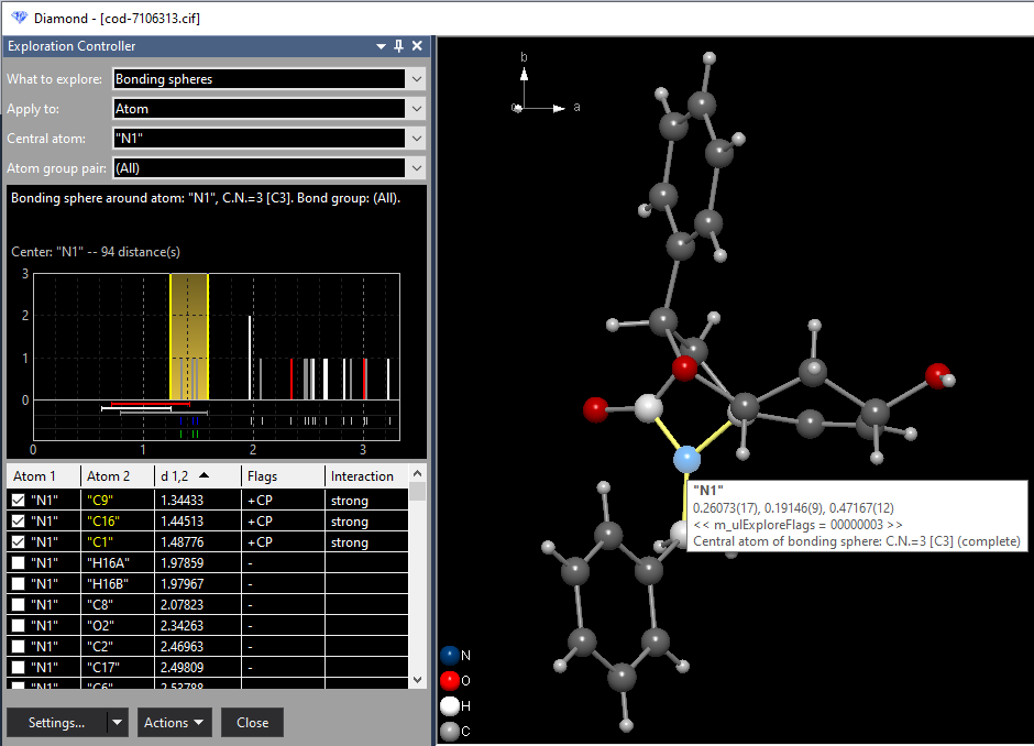
As an example we study the bonding spheres around the atom "N1" by pressing the mouse wheel button or choosing the command Check Bonding Sphere Around Atom "N1" from the context menu, which leads to a situation as depicted in the following. The object of interest "N1" is now listed as "Central atom" in the Exploration Controller.

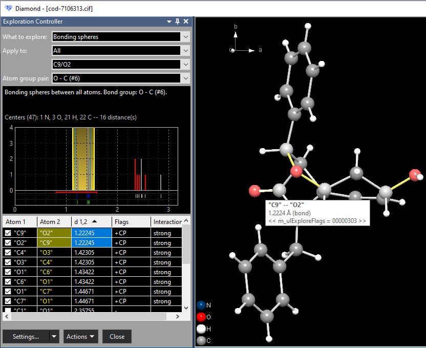
The histogram shows the distances to the neighbouring atoms of "N1", using vertical bars in the neighbouring atoms' atom type colors. The bonding range, i.e. the range between the shortest and longest distance to a bonding neighbouring atom is given in yellow. (There may be multiple bonding ranges, if there is at least a neighouring atom between that is not defined as bonding.)

Below the ground zero line there are multiple horizontal bars defining the bonding spheres as defined in the connectivity. Below the bonding sphere bars, there is a row of ticks for neighbouring atoms inside the Dirichlet domain. Those having strong interaction are given in blue, if they are inside the (blue marked) bonding range - or red if outside. Weak interactions have grey ticks.

If bonding parameters are defined, there is a second and last row, with a tick for every bond defined. A tick is green, if the bond is inside the bonding range, or red otherwise.

The table of neighbouring atoms lists all neighbouring atoms of "N1". The columns show:
- Atom 1: The label of the first atom of the bonding (or contact) sphere, here: the central atom.
- Atom 2: The label of the second atom of the sphere, here the neighbouring atom.
- d 1,2: The distance, in Angstroem, between atom 1 and atom 2.
- Flags: One or more of the following signs:
-- A plus or minus sign indicates that the atom belongs to the atomic environment and corresponds with the checkmark, unless you manually set or clear a checkmark to manually add or remove an atom to or from the atomic environment.
-- 'C' means that the neighbouring atom matches the bonding sphere of the corresponding atom type pair (for instance Sb+3--F-1) in the connectivity.
-- 'D' means that the neighbouring atom belongs to the Dirichlet domain (which does not necessarily mean there is a strong interaction with the central atom, since there are additional conditions for that).
-- 'P' means that the neighbouring atom is defined as bonded to the central atom in the bond parameter list, that means in the structural parameters.
- Interaction: The strength of the interaction, taken from Dirichlet domain calculations and overlap of deriving "spherical domains" and "Slater radii": "strong" for (strongly) bonding interaction, "v.d.W." for weak and "0" or blank for no interaction.

The labels of the bonding neighbouring atoms are given in yellow. If you add another atom to the bonding sphere, this atom's label is given in green. If you remove an atom from the bonding sphere, its label becomes red. Adding and removing of atoms from a bonding sphere is shown in the second example (Sb₄F₁₆) below.

Case 2: Studying bonding spheres between atom types

Now after the - simple example of - studying a bonding sphere around a selected atom, we change to study bonding spheres within the whole molecule or the whole structure picture (which in this example is the same). Here we want to study the C--O bonding spheres as another simple example.

Choose the command Clear Target from the context menu of the graphics view to unselect the current central atom "N1". Move the mouse cursor to a C--O bond, which lights up the grey bond cylinder and shows an info window containing the labels of the connected atoms and the bond length. With the right mouse button, click on this C--O bond and choose the command Check Bonding Spheres: "C--O":

Exploration of bonding spheres between C and O atoms with "Apply to" set to "All". In this example we clicked on the C9 -- O2 bond, so this atom pair is highlighted both in the graphics view as well as in the distances table.

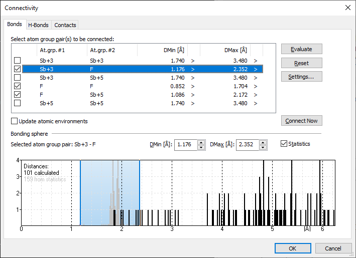
Example antimony trifluoride/pentafluoride adduct (Sb4F16)

Here we use an inorganic compound, an antimony trifluoride/pentafluoride adduct from Pearson's Crystal Data (PCD-1251073), where some of the Sb sites have a wide range of Sb--F distances around the Sb central atom each. We will take a short overview in both the Connectivity and the Atomic Environments dialog, before we switch to the Exploration view.

We open the sample file PCD-1251073.diamdoc, it comes up with a single picture containing all Sb and F atoms inside the unit cell without bonds.

First we stay in the Picture Edit view and run the command Build -> Connectivity, which shows a narrow range for the atom type pair Sb(+5)--F(-1) but a rather wide range for Sb(+3)--F(-1) on the Bonds page of the Connectivity dialog:

Screenshots of Connectivity dialog: Sb(+3)--F(-1) bonding sphere above, Sb(+5)--F(-1) bonding sphere below.

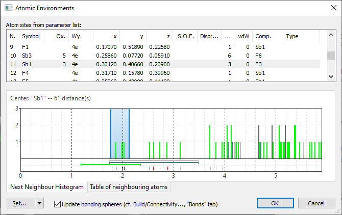
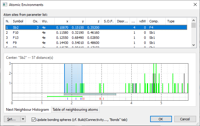
After closing the Connectivity dialog with Cancel and opening the Atomic Environments dialog with the command Build -> Atomic Environments we find a total number of four Sb atom sites, two of them with Sb(+3). The first of them, "Sb1", looks ok in the Next Neighbour Histogram, whereas "Sb2" has a scattering range of Sb--F distances:

Screenshots of Atomic Environments dialog with the two atom sites containing Sb(+3): Atomic environment of "Sb1" above, "Sb2" below.

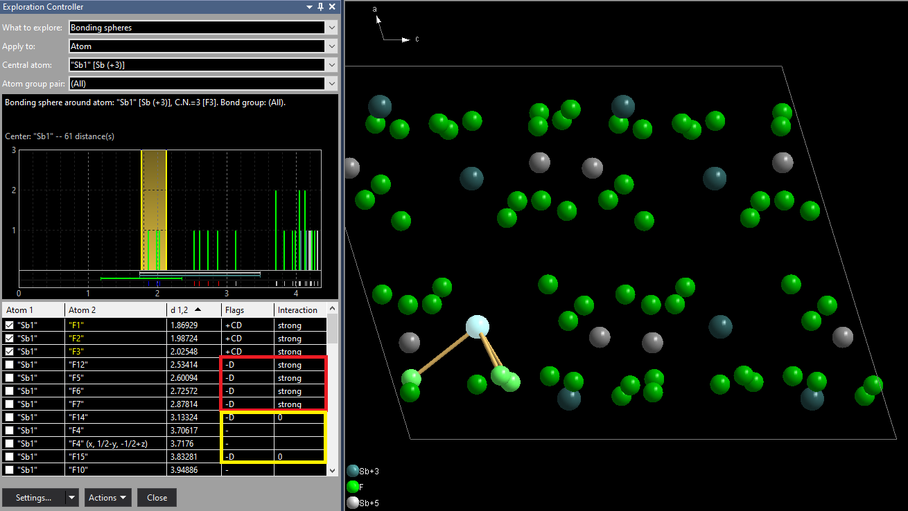
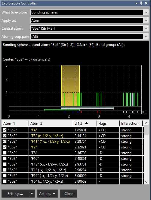
Please note: The atomic environment of this sample compound is described in more detail in the article "Atomic Environments", the determination of atom site environments basing upon Dirichlet domains (Voronoi polyhedra) in "Dirichlet Domains".

After this raw inspection of bonding spheres and atomic environments in the dialogs, we now check this issue in the Exploration view, which allows a higher grade of interaction with the structure picture graphics. We directly enter the exploration with the toolbar button [...]

The site "Sb1" has a rather clear looking next neighbour histogram with a rather big gap between the 3rd and 4th F neighbouring atom. But the distance table tells us there are more strong interactions. The column shows "+CD" flags for the first three Sb--F distances, meaning they are assigned as connected ('+') basing upon the connectivity (C) settings. In more detail: The Sb(+3)--F(-1) bonding sphere has been calculated by Diamond from the sums of the effective radii of Sb(+3) and F(-1) and a factor for the lower sphere boundary of 0.6 and a factor of 1.2 for the upper sphere boundary, leading to a sphere range from 1.176 to 2.352 Å.

But there are four more Sb--F distances in the range between 2.5 and 3.0 Å from the calculation of Dirichlet domains ('D' flag) with strong interactions (red marked). (The yellow marked distances are part of the Voronoi polyhedron but do not contribute to strong interactions ('0' in Interaction column):

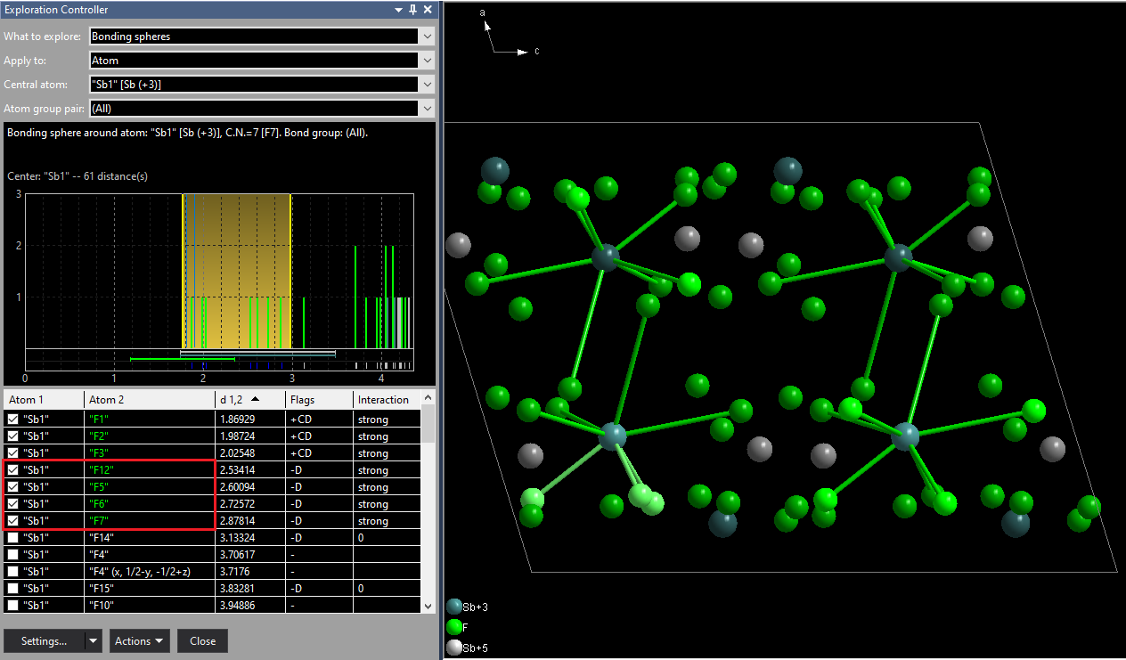
We now add the four F neighbours between 2.5 and 3.0 Å gaining a total coordination number of 7. The easiset way is to shift the upper boundary in the next neighbour histogram to a position of (approx.) 3 Å, an alternative way to set the checkmarks at the four corresponding atoms in the table, that means adding "F12", "F5", "F6", and "F7".

Added neighbours appear green in the distance table and have green Sb--F bonds in the picture. If you decrease the sphere boundary (or clear checkmarks), i.e. remove neighbours, the atoms in the table and the bonds become red instead (here not shown).

In the structure picture neighbouring atoms are created (if not yet present) and connected with the central atom, including symmetry-equivalent atoms. (In this example we have four symmetry-equivalent positions of "Sb1". "Sb1" is on the 4e Wyckoff position.)

[NOTE: Due to a bug in the Preview version the three bonds below 2.5 Å are not created automatically at the three "Sb1" atoms that are symmetry-equivalent to the reference atom "Sb1" at (x, y, z). You should first drag the upper boundary below the shortest Sb-F distance, then re-drag to the 3 Å position.]

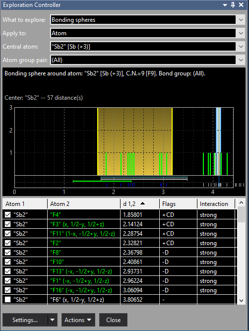
Finally we have a look at the "Sb2" position where the scattering of Sb-F distances is obvious, with the upper sphere boundary at 2.352 Å between 2.328 (Sb2--F2) and 2.368 Å (Sb2--F8). We shift the upper boundary to approx. 3.1 Å resulting in a coordination of 9 F atoms:

Previous article: Working in Exploration View
Next article: Exploring H-bonds and contact spheres

References:
COD:7106313 - Zhongxuan Xu, Kun Huang, Tong Liu, Mingjin Xie, Hongbin Zhang: Synthesis of spirocyclic ?-keto-lactams: copper catalyzed process. Chem.Commun., 47, 4923 (2011).
PCD-1251073 -  Sb₄F₁₆ in P12₁/c1 (14);
"The Crystal Structure of the 1:1 Adduct of Antimony Trifluoride and Antimony Pentafluoride", by: Gillespie R.J., Slim D.R., Vekris J.E.; J. Chem. Soc. (Dalton Trans.) 1977, p. 971.